Lock rows or Columns in Excel

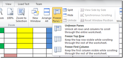
While working on excels with tremendous amount of data, it is desired many a times to track if the current cell alignment is corresponding to right column or to make sure data is entered in a correct cell. This issue arises frequently when the excel worksheet is stuffed with loads of data and in such scenarios user has to scroll left/up and then right/down back to work. To keep an area of a worksheet visible while you scroll to another area of the worksheet, you can lock specific rows or columns in one area by freezing panes .

By freezing the panes, you keep specific rows or columns visible when you scroll in the worksheet. This feature makes important columns display as you move throughout the spreadsheet. Locking columns in Excel is an option called freezing panes.

To lock or freeze Row/Column in an Excel, follow these steps :

1 Open an Excel worksheet. Add data into row and column header as well as in cells as desired.

2 Highlight the entire column/row to lock.

3 Click on the "View" tab if using Microsoft Excel 2010. Under the Window group item in the menu, click on the arrow for "Freeze Panes." Select the option to "Freeze First Column" to lock only the one column highlighted. Select the option to "Freeze Top Row" if you want to freeze the top Row at one time.

4 Repeat the process listed in steps 1 through 3 and then select “Unfreeze Panes” to unlock all the panes .

And the Row/Column locked, scrollable Excel sheet is prepared. Quiet handy in the worksheets dealing with enormous amounts of data.